Hybrid Artificial Intelligence Machines As Creative Partners Training Ppt
This training module on Hybrid Artificial Intelligence Machines as Creative Partners introduces the concept of hybrid artificial intelligence along with its pros and cons. It also provides an in-depth understanding of Artificial Neural Networks ANN by explaining the layers, neurons, and various functions Activation, Threshold, Sigmoid, Rectifier, Hyperbolic Tangent. It also informs about the working, advantages and disadvantages of ANN, gradient descent, and backpropagation. It also presents information about Convolutional Neural Network CNN, its working, and its layers. Further, it tells us about autoencoders, variational autoencoders, feedforward neural networks, and recurrent neural networks. It also discusses the mixture density network. It also includes Key Takeaways and Discussion Questions related to the topic to make the training session more interactive. The deck has PPT slides on About Us, Vision, Mission, Goal, 30-60-90 Days Plan, Timeline, Roadmap, Training Completion Certificate, and Energizer Activities. It also includes a Client Proposal and Assessment Form for training evaluation.
- Google Slides is a new FREE Presentation software from Google.
- All our content is 100% compatible with Google Slides.
- Just download our designs, and upload them to Google Slides and they will work automatically.
- Amaze your audience with SlideTeam and Google Slides.
-
Want Changes to This PPT Slide? Check out our Presentation Design Services
- WideScreen Aspect ratio is becoming a very popular format. When you download this product, the downloaded ZIP will contain this product in both standard and widescreen format.
-

- Some older products that we have may only be in standard format, but they can easily be converted to widescreen.
- To do this, please open the SlideTeam product in Powerpoint, and go to
- Design ( On the top bar) -> Page Setup -> and select "On-screen Show (16:9)” in the drop down for "Slides Sized for".
- The slide or theme will change to widescreen, and all graphics will adjust automatically. You can similarly convert our content to any other desired screen aspect ratio.
Compatible With Google Slides

Get This In WideScreen
You must be logged in to download this presentation.
PowerPoint presentation slides
Presenting Training Deck on Unlocking the Fundamentals of NLP, NLU, and NLG. This deck comprises of 113 slides. Each slide is well crafted and designed by our PowerPoint experts. This PPT presentation is thoroughly researched by the experts, and every slide consists of appropriate content. All slides are customizable. You can add or delete the content as per your need. Not just this, you can also make the required changes in the charts and graphs. Download this professionally designed business presentation, add your content, and present it with confidence.
People who downloaded this PowerPoint presentation also viewed the following :
Content of this Powerpoint Presentation
Slide 4
This slide introduces the concept of Hybrid Artificial Intelligence. Hybrid AI is a breakthrough that blends non-symbolic AI, such as machine learning and deep learning systems, with symbolic AI or human intelligence embedded in machines
Slide 5
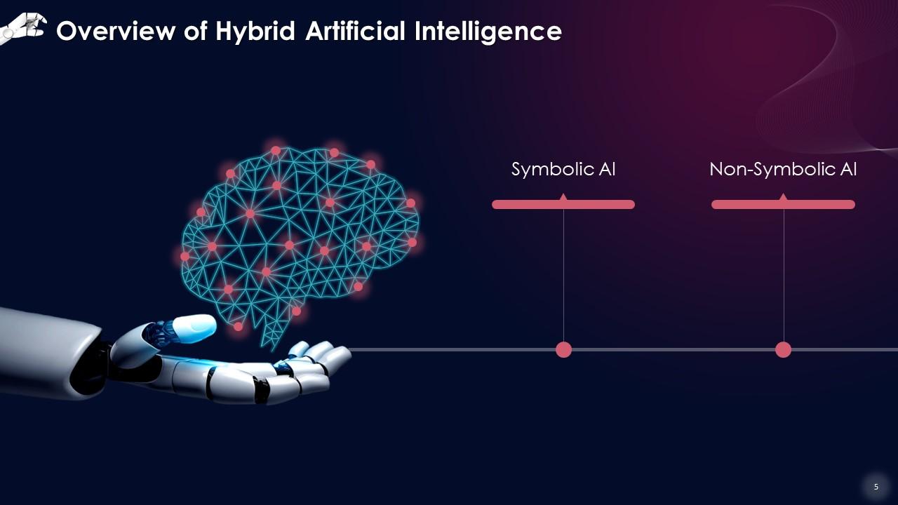
This slide describes the two areas of Artificial Intelligence that are, Symbolic AI and Non-Symbolic AI. These two areas are the main pillars of Hybrid Artificial Intelligence.
Instructor’s Notes:
- Symbolic AI: Symbolic AI attempts to connect facts and occurrences using logic rules and make this information machine-readable and retrievable through semantic enrichment
- Non-Symbolic AI: This category comprises models in Machine Learning, Deep Learning, and neural networks, where a large amount of training data is used to get statistical inferences and judgments. This is also true when we submit a text to the Natural Language Understanding (NLU) component, which understands it and returns the correct response
Slide 6
This slide lists the advantages and disadvantages of using hybrid AI models. The pros include a strong and robust model, and the flexibility it offers. The cons include complexity to understand, hard to implement, and its training intensive nature.
Slide 7
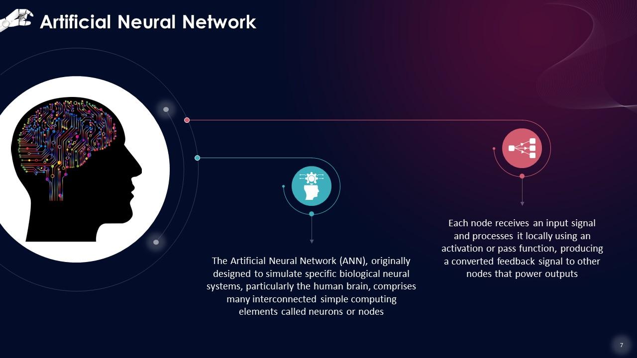
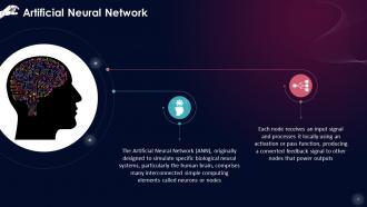
This slide gives an overview of Artificial Neural Network. It is designed to simulate specific biological neural systems, particularly the human brain, and comprises many interconnected simple computing elements called neurons or nodes.
Slide 8
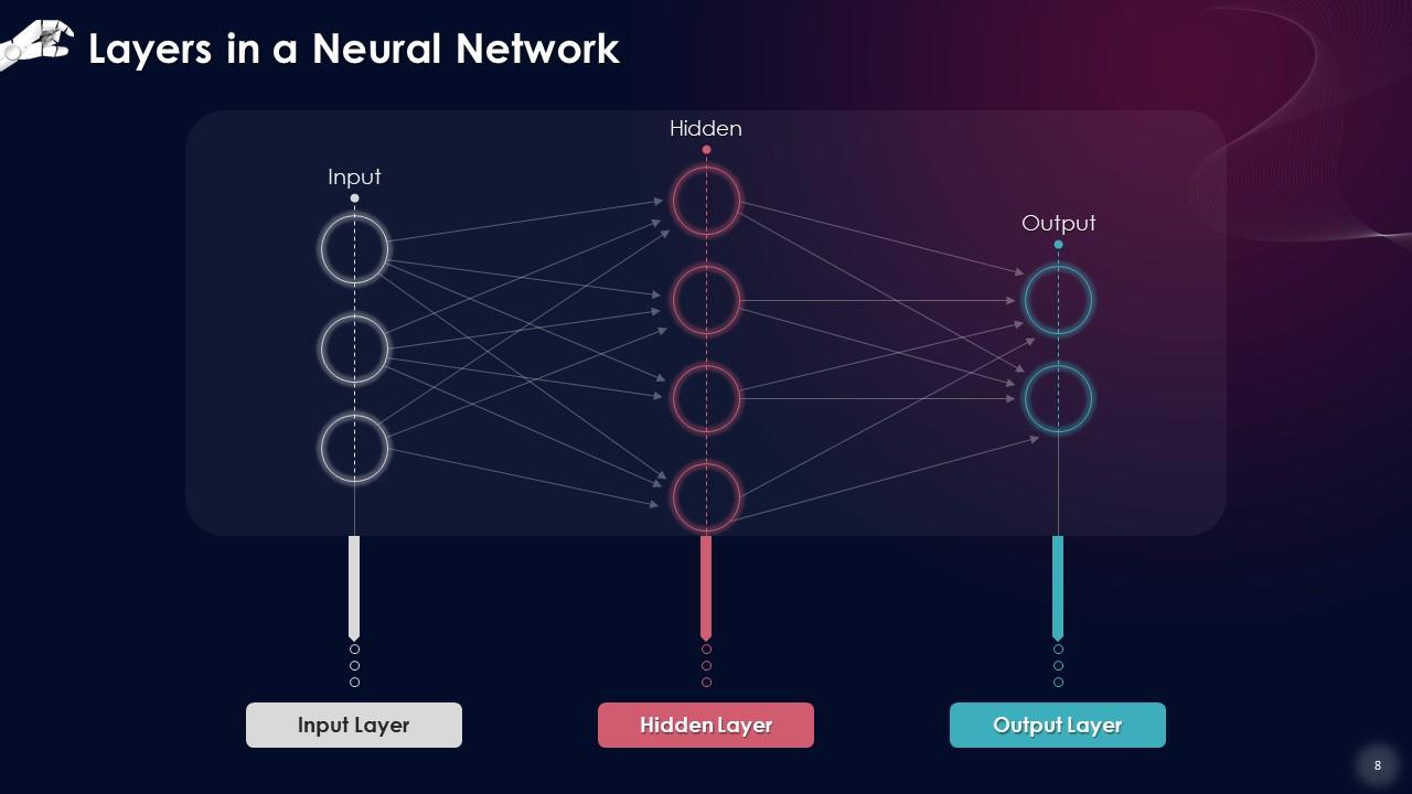
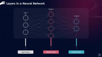
This slide depicts the layers in a Neural network. There are three layers known as the input layer, hidden layer, and output layer.
Instructor’s Notes:
- Input Layer: The input layer comes first. This layer will accept the data, which will then send it to the remainder of the network
- Hidden Layer: The hidden layer is the second of the three layers. A neural network’s hidden layers can be one or more in number. The hidden layers are the ones that are accountable for neural networks' high performance and complexity. They may do a number of tasks at once, such as data transformation, automatic feature development, etc
- Output Layer: The output layer is the final layer. The outcome or output of the problem is stored in the output layer. The input layer receives raw photos, and the output layer delivers the final version of the result
Slide 9
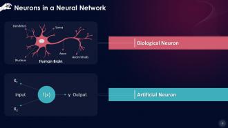
This slide illustrates the artificial neurons present in the layers of an Artificial Neural Network (ANN). It draws a comparison between the biological neurons present in human brains with an artificial neuron in an ANN.
Instructor’s Notes: A layer is made up of microscopic units known as neurons. A neuron in a neural network can be better understood with the help of biological neurons. An artificial neuron is analogous to a biological neuron. It takes information from other neurons, processes it, and then produces an output. Here, X1 and X2 are the artificial neurons' inputs, f(X) is the processing done on the inputs, and y is the neuron's output.
Slide 10
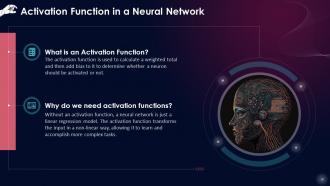
This slide gives an introduction to activation function in a neural network and discusses its importance. The activation function is used to calculate a weighted total and then add bias to it to determine whether a neuron should be activated or not.
Slide 11
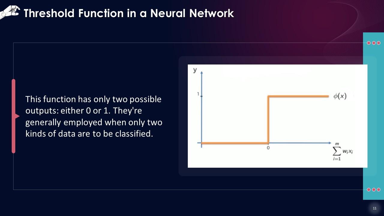
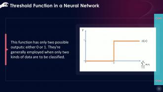
This slide illustrates Threshold Function which is a type of Activation Function in a neural network. This function has only two possible outputs: either 0 or 1. They're generally employed when only two kinds of data are to be classified.
Slide 12
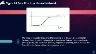
This slide depicts Sigmoid Function which is a type of activation function. The range of values for the sigmoid function is 0 to 1. This function is primarily employed in the output layer because it is from this node that we obtain the anticipated value
Slide 13
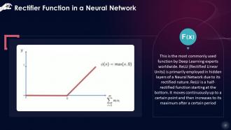
This slide illustrates Rectifier or ReLU function which is a type of activation function. Relu (Rectified Linear Units) is primarily employed in hidden layers of a Neural Network due to its rectified nature. Relu is a half-rectified function starting at the bottom. It moves continuously up to a certain point and then increases to its maximum after a certain period
Slide 14
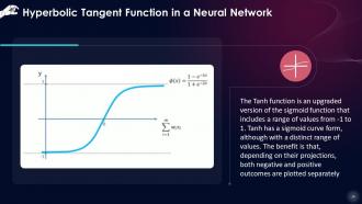
This slide depicts Hyperbolic Tangent Function which is a type of activation function. The Tanh function is an upgraded version of the sigmoid function that includes a range of values from -1 to 1. Tanh has a sigmoid curve form, although with a distinct range of values. The benefit is that, depending on their projections, both negative and positive outcomes are plotted separately
Slide 15
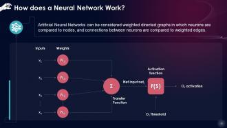
This slide describes the working of an Artificial Neural Network. Artificial Neural Networks can be considered weighted directed graphs in which neurons are compared to nodes, and connections between neurons are compared to weighted edges.
Instructor’s Notes: A neuron's processing element receives many signals, which are occasionally altered at the receiving synapse before being summed at the processing element. If it reaches the threshold, it becomes an input to other neurons, and the cycle begins again
Slide 16
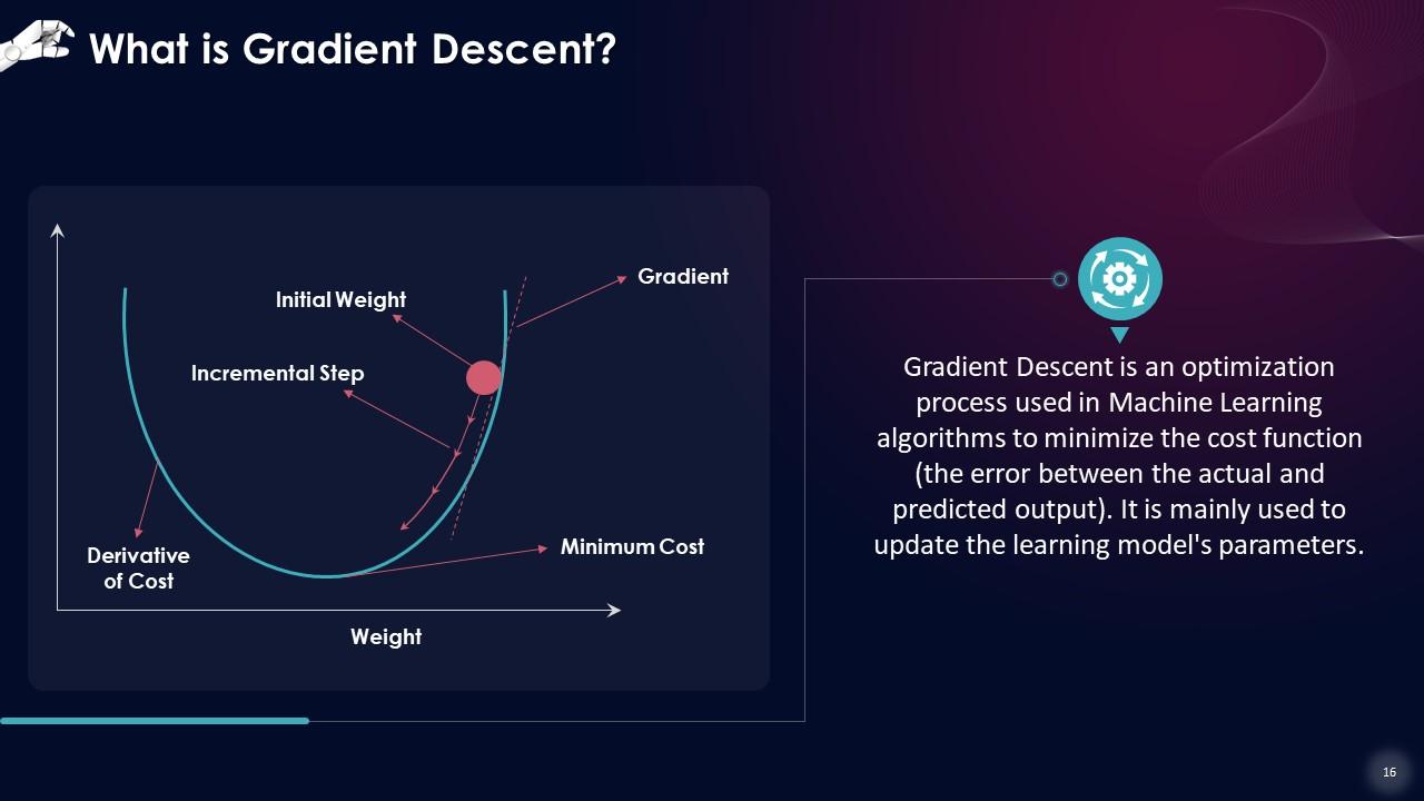
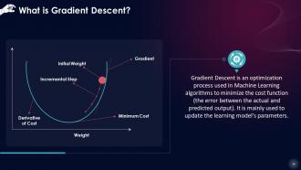
This slide introduces the concept of gradient descent. Gradient Descent is an optimization process used in Machine Learning algorithms to minimize the cost function (the error between the actual and predicted output). It is mainly used to update the learning model's parameters.
Slide 17
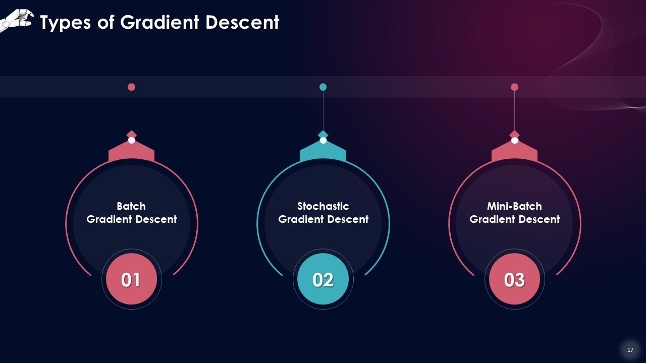
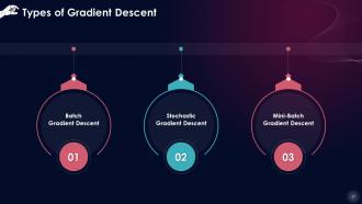
This slide lists types of gradient descent. These include batch gradient descent, stochastic gradient descent, and mini-batch gradient descent.
Instructor’s Notes:
- Batch Gradient Descent: Batch gradient descent adds the errors for each point in a training set before updating the model after all training instances have been reviewed. This process is known as the Training Epoch. Batch gradient descent usually gives a steady error gradient and convergence, although choosing the local minimum rather than the global minimum isn't always the best solution
- Stochastic Gradient Descent: Stochastic gradient descent creates a training epoch for each example in the dataset and changes the parameters of each training example, sequentially. These frequent updates can provide greater detail and speed, but they can also produce noisy gradients, which can aid in surpassing the local minimum and locating the global one
- Mini-Batch Gradient Descent: Mini-batch gradient descent combines the principles of both batch gradient descent with stochastic gradient descent. It divides the training dataset into distinct groups and updates them separately. This method balances batch gradient descent's computing efficiency and stochastic gradient descent's speed
Slide 18
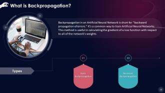
This slide describes the concept of backpropagation along with its two types that are Static backpropagation and Recurrent backpropagation. Backpropagation is useful in calculating the gradient of a loss function with respect to all of the network's weights.
Instructor’s Notes:
- Static Backpropagation: The mapping of static input generates a static output in this type of backpropagation. It is used to address challenges like optical character recognition that requires static classification
- Recurrent Backpropagation: The Recurrent Propagation is directed forward or conducted till a specific set value, or threshold value is attained. The error is evaluated and propagated backward after reaching a particular value
Slide 19
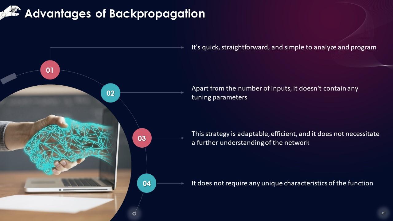
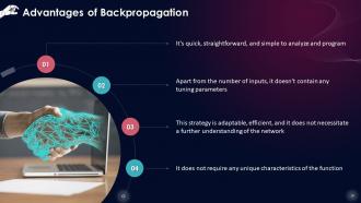
This slide lists the advantages of Backpropagation. These are that it is simple & straightforward, adaptable & efficient, and it does not require any unique characteristics.
Slide 20
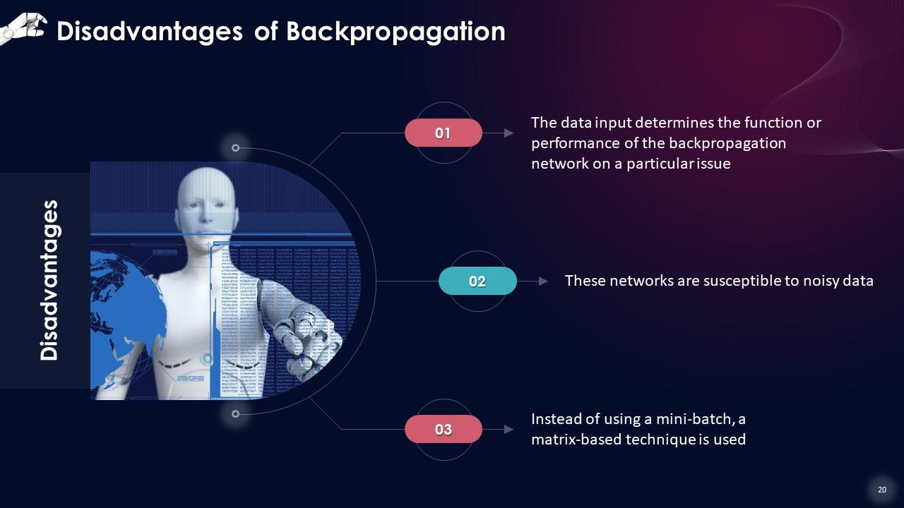
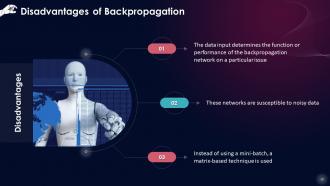
This slide lists the disadvantages of Backpropagation. These are that the data input determines the function of the entire network on a particular issue, networks are susceptible to noisy data, and a matrix based technique is used.
Slide 21
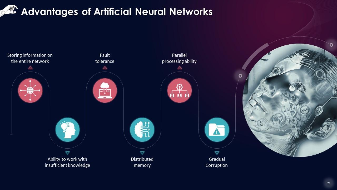
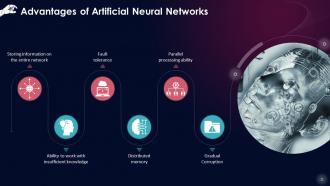
This slide lists the advantages of Artificial Neural Networks. These advantages include that ANN stores information on the entire network, its ability to work with insufficient knowledge, its fault tolerance, a distributed memory, and parallel processing ability.
Instructor’s Notes:
- Storing information on the entire network: Information is saved on the entire network, not in a database, as done in traditional programming. The network continues to function despite losing a few pieces of information in one location
- Ability to work with insufficient knowledge: After training the Artificial Neural Network, the data can yield output even with limited or insufficient information
- Fault tolerance: The output of an ANN is unaffected by the corruption of one or more of its cells. The networks become fault-tolerant as a result of this characteristic
- Distributed memory: It is required to determine the examples and train the network according to the intended output. The network's progress is proportional to the instances chosen. If the event cannot be displayed to the network in all aspects, it may generate inaccurate results
- Parallel processing ability: Artificial Neural Networks have the computational power to perform multiple tasks at once
- Gradual Corruption: The network is not immediately corroded as its performance degrades and slows over time.
Slide 22
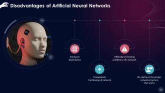
This slide lists the disadvantages of Artificial Neural Networks. These disadvantages include ANNs’ hardware dependence, unexplained functioning of network, difficulty of showing problem to the network, and no clarity on the proper network structure that works.
Instructor’s Notes:
- Hardware dependence: The structure of Artificial Neural Networks necessitates parallel processing power. As a result, the implementation is equipment dependent
- Unexplained functioning of network: When ANN provides a probing solution, it does not explain why or how it was chosen. This decreases trust in the network
- Difficulty of showing problem to the network: ANNs are able to work with numerical data. Before introducing ANN to a problem, it must be transformed into numerical values. The display mechanism chosen here will directly impact the network's performance, depending on the user's skill level
- No clarity on the proper network structure that works: No explicit rule determines the structure of artificial neural networks. Experience and trial & error are used to create the ideal network structure
Slide 24
This slide gives an overview of Convolutional Neural Networks. ConvNet, is a deep learning network design that learns from data without the requirement for human feature extraction. CNNs are beneficial for recognizing objects, faces, and settings by looking for patterns in images.
Slide 25
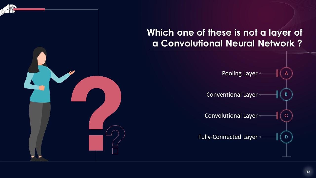
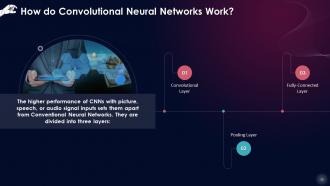
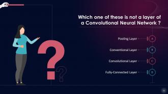
This slide describes how Convolutional Neural Networks work. CNNs are divided into three layers that are convolutional layer, pooling layer, and fully-connected layer.
Slide 26
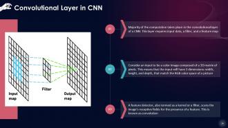
This slide depicts the Convolutional Layer in a Convolutional Neural Network. The majority of the computation takes place in the convolutional layer of a CNN. This layer requires input data, a filter, and a feature map.
Slide 27
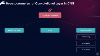
This slide describes hyperparameters of the Convolution layer in a CNN. These parameters are number of filters, stride, and zero-padding which is further divided into valid padding, same padding, and full padding.
Instructor’s Notes:
- Number of filters: The depth of the output is determined by the amount of filters used. Three distinct filters, for instance, would result in three distinct feature maps, resulting in a depth of three
- Stride: The stride of the kernel is the number of pixels traversed over the input matrix. Despite the fact that stride values of two or more are unusual, a longer stride means less output
- Zero-padding: Zero-padding is used when the filters don't fit the input image. All members outside the input matrix are set to zero, resulting in a larger or equal-sized output. Padding is of three types
- Valid padding: This is also referred to as "no padding." If the dimensions do not align, the last convolution is discarded
- Same padding: This padding guarantees that the size of the output layer and input layer is the same
- Full padding: This type of padding enhances the output's size, By padding the input's border with zeros
Slide 28
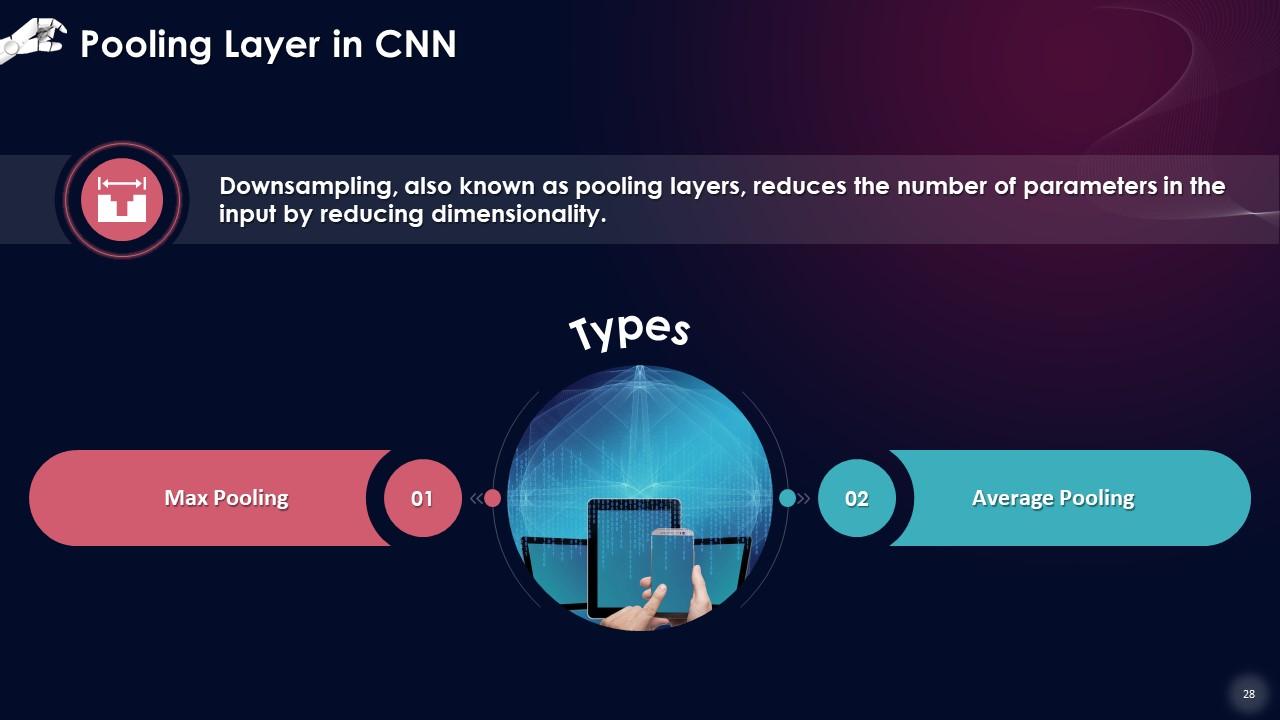
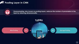
This slide depicts the Pooling Layer in a Convolutional Neural Network. Downsampling, also known as pooling layers, reduces the number of parameters in the input by reducing dimensionality. Max Pooling and Average Pooling are its two types.
Instructor’s Notes: The pooling process sweeps a filter across the entire input, similar to the convolutional layer, except that this filter has no weights. Instead of populating the output array with values from the receptive field, the kernel uses an aggregation function.
- Max Pooling: The filter chooses the pixel with the highest value to transmit to the output array as it advances across the input. In comparison to average pooling, this strategy is employed more frequently
- Average Pooling: The average value inside the receptive field is determined as the filter passes over the input and is sent to the output array
Slide 29
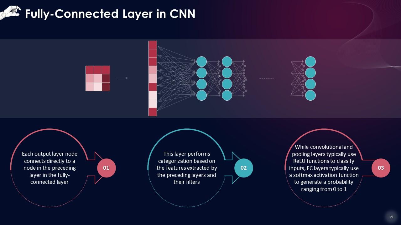
This slide depicts the Fully-Connected Layer in a Convolutional Neural Network. Each output layer node connects directly to a node in the preceding layer in the fully-connected layer. This layer performs categorization based on the features extracted by the preceding layers and their filters
Slide 30
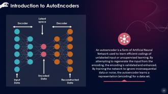
This slide gives an overview of AutoEncoders in Neural Networks. An Autoencoder is a form of Artificial Neural Network used to learn efficient codings of unlabeled input or unsupervised learning. By attempting to regenerate the input from the encoding, the encoding is validated and enhanced.
Slide 31
This slide lists components in an AutoEncoder. These components are an encoder, decoder, and latent space.
Instructor’s Notes:
- Encoder: Learns to convert incoming data into an encoded representation by compressing (reducing) it
- Decoder: Recovers the original data from the encoded representation as close as possible to the original input
- Latent space: The layer that includes the compressed version of the input data is known as the bottleneck or latent space
Slide 32
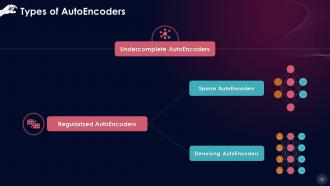
This slide depicts types of AutoEncoders. These include undercomplete Autoencoders and regularized Autoencoders which are further divided into sparse Autoencoders and denoising Autoencoders.
Instructor’s Notes:
- Undercomplete Autoencoders: Undercomplete Autoencoders have a latent space that is smaller than the input dimension. The autoencoder is forced to capture the most important aspects of the training input by learning an incomplete representation
- Regularized Autoencoders: These employ a loss function that promotes the model to have qualities other than the capacity to transfer input to output. Two forms of regularised autoencoders are found in practice: sparse autoencoders and denoising autoencoders
- Sparse Autoencoders: Typically, Sparse Autoencoders are used to learn features for a new job, such as classification. Instead of just operating as an identity function, an Autoencoder that has been regularised to be sparse must respond to unique statistical properties of the dataset it has been trained on
- Denoising Autoencoders: It is no longer necessary to rebuild the input data. Rather than adding a penalty to the loss function, we can change the reconstruction error term of the loss function to obtain an Autoencoder that has the capacity to learn anything meaningful. This can be accomplished by introducing noise to the input image and training the Autoencoder to eliminate it. The encoder will learn a robust representation of the data by extracting the most relevant features
Slide 33
This slide lists applications of AutoEncoders. These include noise removal, dimensionality reduction, anomaly detection, and machine translation.
Instructor’s Notes:
- Noise Removal: The technique of reducing noise from an image is known as noise removal. Audio and picture noise reduction techniques are available through autoencoders
- Dimensionality Reduction: The transfer of data from a high-dimensional space to a low-dimensional space so that the low-dimensional representation retains some significant aspects of the original data, ideally close to its intrinsic dimension, is known as dimensionality reduction. The encoder section of autoencoders is helpful while performing dimensionality reduction since it learns representations of your input data with considerably reduced dimensionality
- Anomaly Detection: The model is encouraged to learn to exactly recreate the most often seen traits by learning to replicate the most salient features in the training data (under some limitations, of course). When confronted with abnormalities, the model's reconstruction performance should deteriorate. In most circumstances, the autoencoder is trained using only data containing normal instances. The autoencoder will correctly reconstruct "normal" data after training but will fail to do so with unexpected anomalous input
- Machine Translation: Autoencoders have been used in Neural Machine Translation (NMT), a type of machine translation that uses autoencoders. Unlike standard autoencoders, the output is not in the same language as the input. Texts in NMT are viewed as sequences to be encoded into the learning mechanism, whereas sequences in the target language(s) are generated on the decoder side
Slide 34
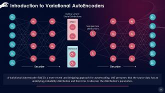
This slide gives an overview of Variational AutoEncoders in Neural Networks. A Variational Autoencoder (VAE) is a more recent and intriguing approach for autoencoding. VAE presumes that the source data has an underlying probability distribution and then tries to discover the distribution's parameters.
Instructor’s Notes: It's far more challenging to implement a Variational Autoencoder than to implement an Autoencoder. A Variational Autoencoder's principal purpose is to generate new data connected to the original source data
Slide 35
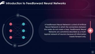
This slide gives an introduction to Feedforward Neural Networks. A Feedforward Neural Network is a kind of Artificial Neural Network in which the connections between the nodes do not create a loop. Feedforward Neural Networks are sometimes described as a multi-layered network of neurons because all information travels forward only.
Slide 37
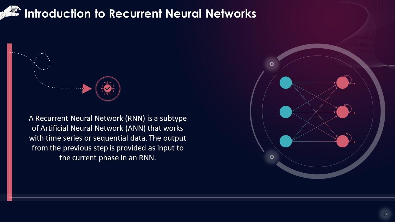
This slide gives an introduction to Recurrent Neural Networks. A Recurrent Neural Network (RNN) is a subtype of Artificial Neural Network (ANN) that works with time series or sequential data. The output from the previous step is provided as input to the current phase in an RNN.
Slide 38
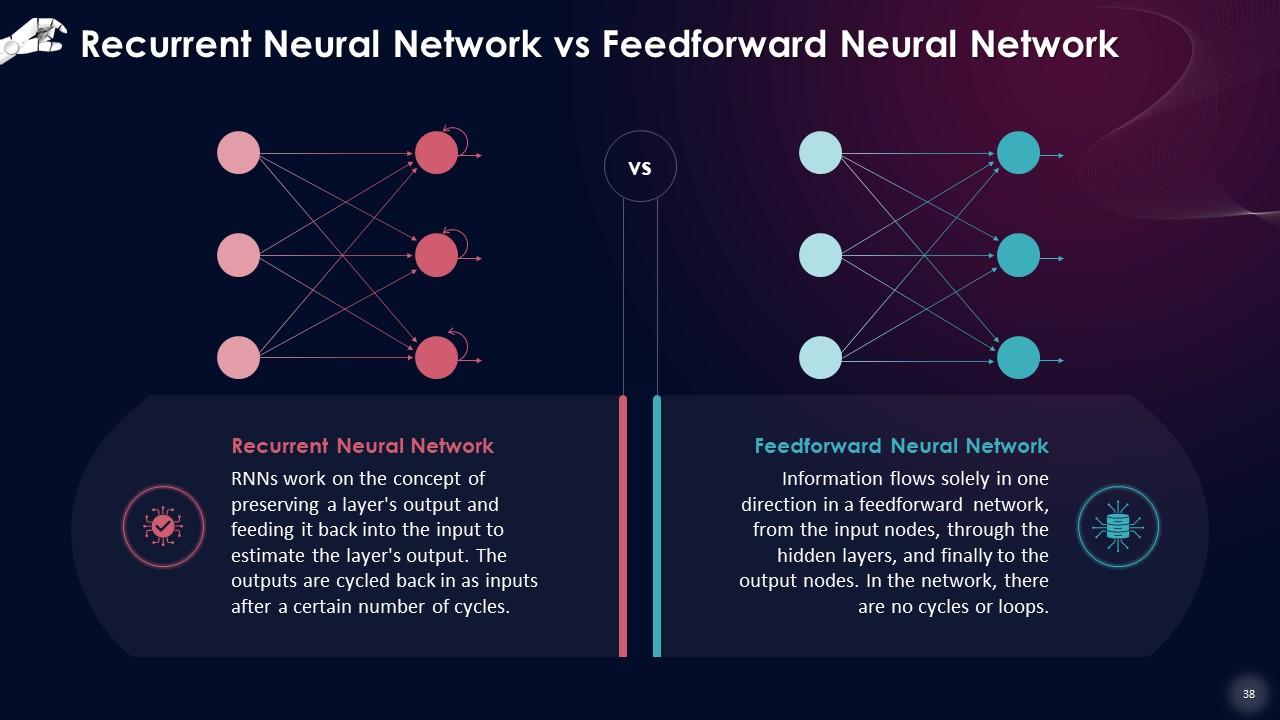
This slide defines a Recurrent Neural Network and a Feedforward Neural Network. RNNs work on the concept of preserving a layer's output and feeding it back into the input to estimate the layer's output.The outputs are cycled back in as inputs after a certain number of cycles. Information flows solely in one direction in a feedforward network, from the input nodes, through the hidden layers, and finally to the output nodes.
Slide 39
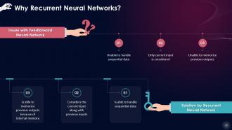
This slide draws a comparison between a Recurrent Neural Network and a Feedforward Neural Network by presenting solutions that RNNs bring to the issues faced by feedforward networks.
Slide 40
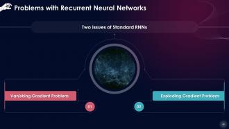
This slide talks about the two issues that standard RNNs present. These are the vanishing gradient problem, and exploding gradient problem.
Instructor’s Notes:
- Vanishing Gradient Problem: Gradients of the loss function approach zero when more layers with certain activation functions are added to neural networks, which makes the network difficult to train.
- Exploding Gradient Problem: An Exploding Gradient occurs when the slope of a neural network grows exponentially instead of diminishing after training. This problem occurs when significant error gradients build up, resulting in extensive modifications to the neural network model weights during training. The main challenges in gradient problems are extended training times, low performance, and poor accuracy
Slide 41
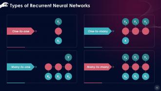
This slide lists types of Recurrent Neural Networks. These include one-to-one, one-to-many, many-to-one, many-to-many.
Slide 42
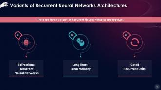
This slide depicts three variants of Recurrent Neural Networks architectures. These include bidirectional recurrent neural networks, long short-term memory, and gated recurrent units.
Slide 43
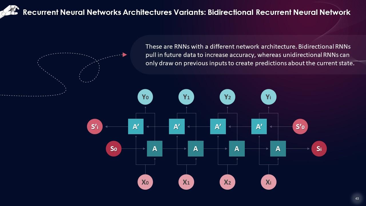
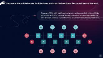
This slide talks about Bidirectional Recurrent Neural Network as an architecture. Bidirectional RNNs pull in future data to increase accuracy, whereas unidirectional RNNs can only draw on previous inputs to create predictions about the current state.
Slide 44
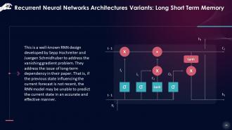
This slide gives information about Long Short Term Memory as an architecture. LSTM is a well-known RNN design developed by Sepp Hochreiter and Juergen Schmidhuber to address the vanishing gradient problem.
Instructor’s Notes: In the deep layers of the neural network, LSTMs have "cells" that have three gates: input gate, output gate, and forget gate. These gates regulate the flow of data required to forecast the network's output.
Slide 45
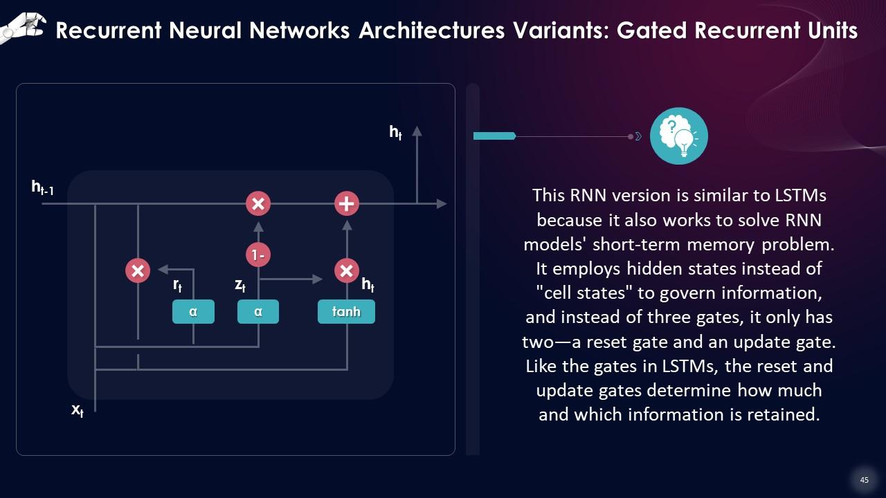
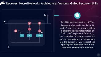
This slide talks about Gated Recurrent Units as an architecture. This RNN version is similar to LSTMs because it also works to solve RNN models' short-term memory problem. It employs hidden states instead of "cell states" to govern information, and instead of three gates, it only has two—a reset gate and an update gate.
Slide 46
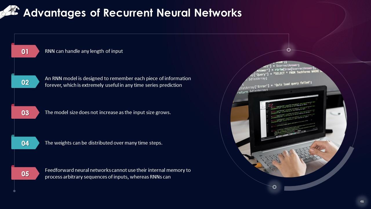
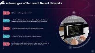
This slide lists advantages of Recurrent Neural Networks. These benefits are that RNNs can handle any length of input, they remember information, the model size does not increase as the input size grows, the weights can be distributed, etc.
Slide 47
This slide lists disadvantages of Recurrent Neural Networks. The drawbacks are that the computation is slow, models can be challenging to train, and exploding and vanishing gradient problems are common.
Slide 48
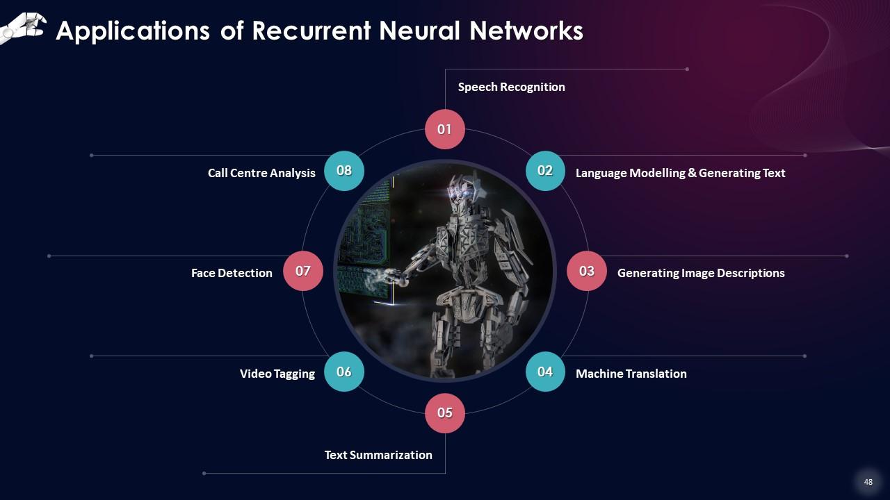
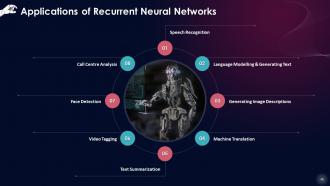
This slide lists applications of Recurrent Neural Networks. These are speech recognition, language modelling & generating text, generating image descriptions, machine translation, text summarization, video tagging, face detection, and call centre analysis.
Instructor’s Notes:
- Speech Recognition: When sound waves from a medium are employed as an input source, RNNs can be used to forecast phonetic segments. The set of inputs comprises phonemes or acoustic signals from an audio file that have been adequately processed and used as inputs
- Language Modelling & Generating: RNNs try to anticipate the potential of the next word using a sequence of words as input. This is one of the most helpful ways of translation since the most likely sentence will be the correct one. The likelihood of a given time-output step is used to sample the words in the next iteration in this method
- Generating Image Descriptions: A combination of CNNs and RNNs is used to describe what is happening inside an image. The segmentation is done using CNN, and the description is recreated by RNN using the segmented data
- Machine Translation: RNNs can be used to translate text from one language to another in one way or the other. Almost every translation system in use today employs some form of advanced RNN. The source language can be used as the input, and the output will be in the user's preferred target language
- Text Summarization: This application can help a lot with summarizing content from books and customizing it for distribution in applications that can't handle vast amounts of text
- Video tagging: RNNs can be used in video search to describe the visual of a video divided into many frames
- Face Detection: Image recognition is one of the simplest RNNs to understand. The method is built around taking one unit of an image as input and producing the image's description in several groups of output
- Call Centre Analysis: The entire procedure can be automated if RNNs are used to process and synthesize actual speech from the call for analysis purposes
Slide 49
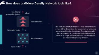
This slide gives an introduction to Mixture Density Networks. A Mixture Density Network is an interesting model for working on supervised learning issues where a single standard probability distribution cannot represent the target variable. It is created within the basic framework of neural networks and probability theory.
Instructor’s Notes: In essence, an MDN allows you to model a conditional probability distribution p(y|x) as a mixture of distributions, with the individual distributions and mixing coefficients defined by functions of the inputs x.
Slide 50
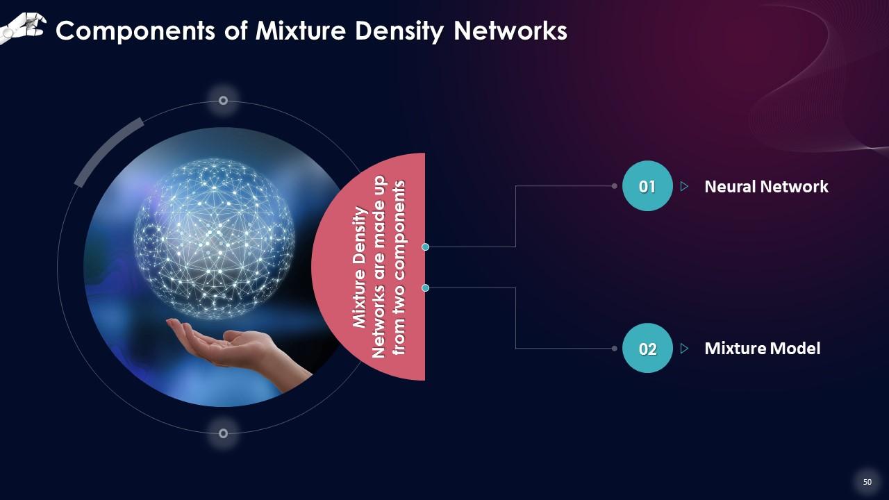
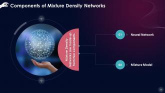
This slide depicts the two components that a Mixture Density Network is made of. These are a neural network and a mixture model
Instructor’s Notes:
- Neural Network: Any viable architecture that takes the input X and converts it into a set of learned features is a Neural Network (we can think of it as an encoder or backbone)
- Mixture Model: The Mixture Model is a probability distribution model composed of a weighted sum of simpler distributions
Slide 51
This slide shows how a Mixture Density Network looks like. The Mixture Density Network is a feed-forward neural network that determines the parameters of a mixture density model using its outputs.
Slide 67 to 82
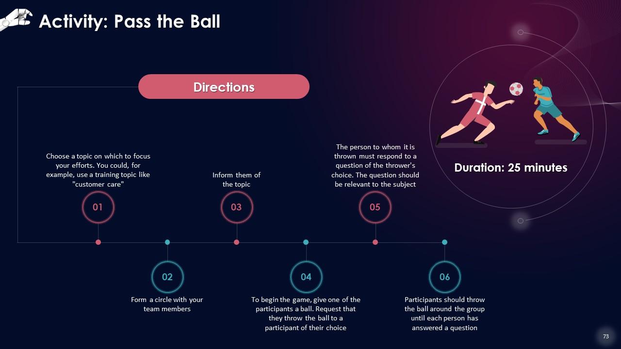
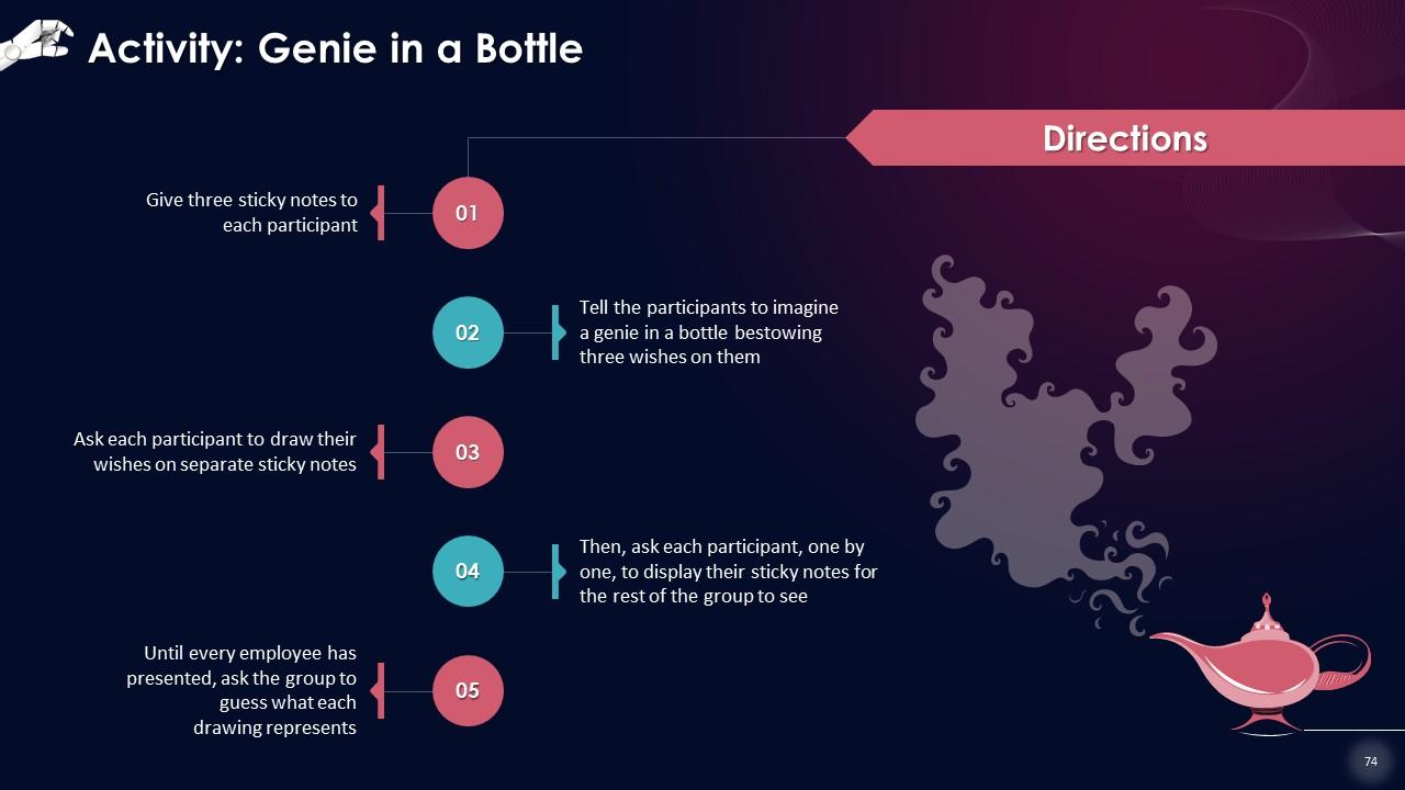
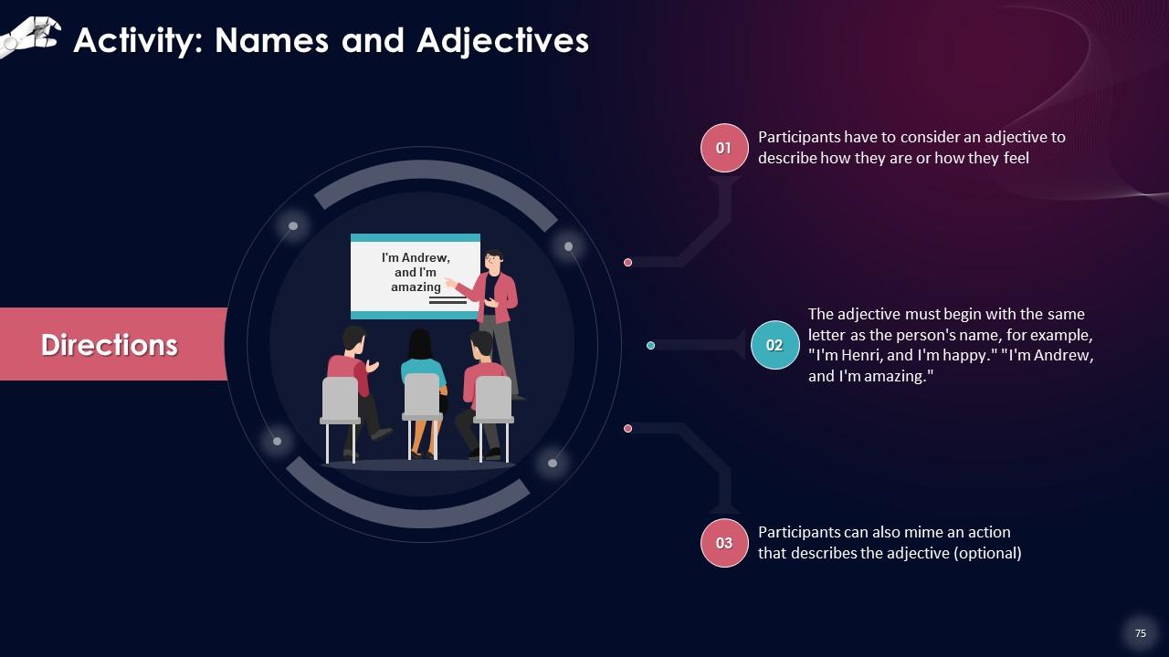
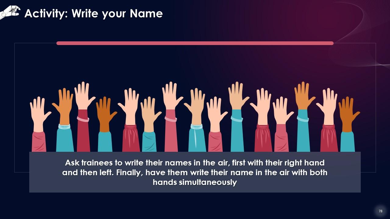
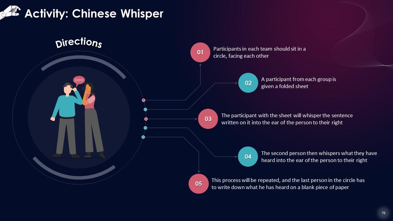
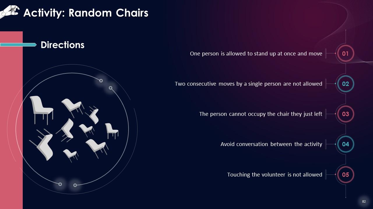
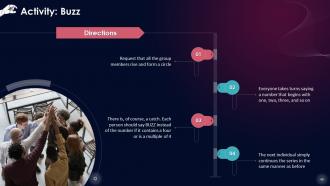
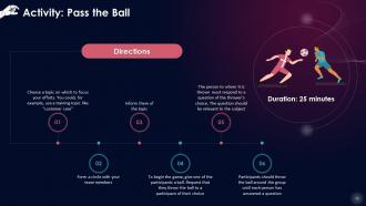
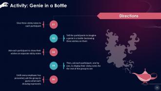
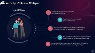
These slides contain energizer activities to engage the audience of the training session.
Slide 83 to 110
These slides contain a training proposal covering what the company providing corporate training can accomplish for the client.
Slide 111 to 113
These slides include a training evaluation form for instructor, content and course assessment.
Hybrid Artificial Intelligence Machines As Creative Partners Training Ppt with all 118 slides:
Use our Hybrid Artificial Intelligence Machines As Creative Partners Training Ppt to effectively help you save your valuable time. They are readymade to fit into any presentation structure.
-
Unique and attractive product design.
-
The team is highly dedicated and professional. They deliver their work on time and with perfection.


