Core Functions Of Deep Learning Training Ppt
These slides explain the functions of Deep Learning. They are Sigmoid Activation Function, tan-h Hyperbolic Tangent Function, ReLU Rectified Linear Units, Loss Functions, and Optimizer Functions. The Loss Function further includes Mean Absolute Error, Mean Squared Error, Hinge Loss, and Cross-Entropy.
You must be logged in to download this presentation.
 Impress your
 audience
Editable
of Time
PowerPoint presentation slides
Presenting Core Functions of Deep Learning. These slides are 100 percent made in PowerPoint and are compatible with all screen types and monitors. They also support Google Slides. Premium Customer Support available. Suitable for use by managers, employees, and organizations. These slides are easily customizable. You can edit the color, text, icon, and font size to suit your requirements.
People who downloaded this PowerPoint presentation also viewed the following :
Content of this Powerpoint Presentation
Slide 1
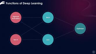
This slide states multiple types of Deep Learning functions: Sigmoid Activation Function, tan-h (Hyperbolic Tangent Function), ReLU (Rectified Linear Units), Loss Functions, and Optimizer Functions.
Slide 2
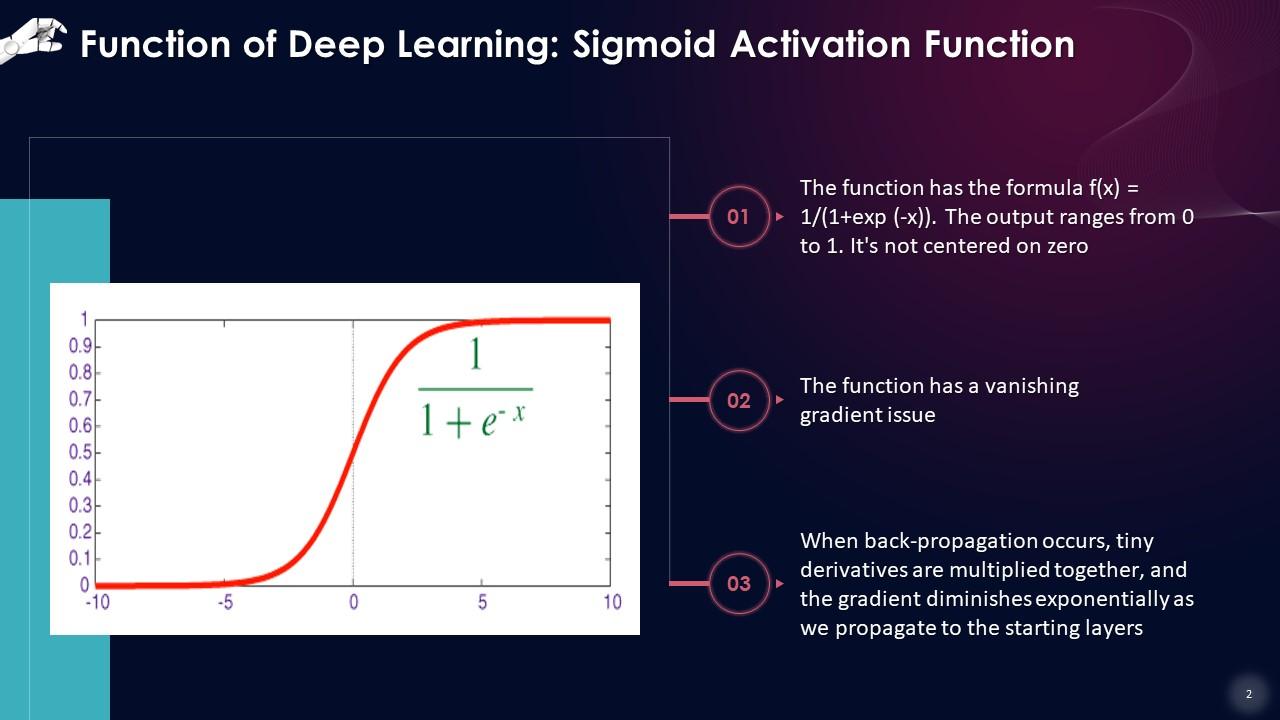
This slide gives an overview of sigmoid activation function which has the formula f(x) = 1/(1+exp (-x)). The output ranges from 0 to 1. It's not centered on zero. The function has a vanishing gradient issue. When back-propagation occurs, tiny derivatives are multiplied together, and the gradient diminishes exponentially as we propagate to the starting layers.
Slide 3
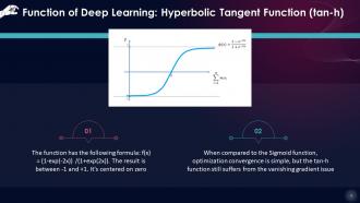
This slide states that Hyperbolic Tangent function has the following formula: f(x) = (1-exp(-2x))/(1+exp(2x)). The result is between -1 and +1. It's centered on zero. When compared to the Sigmoid function, optimization convergence is simple, but the tan-h function still suffers from the vanishing gradient issue.
Slide 4
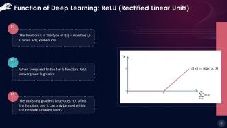
This slide gives an overview of ReLU (Rectified Linear Units). The function is in the type of f(x) = max(0,x) i,e 0 when x<0, x when x>0. When compared to the tan-h function, ReLU convergence is greater. The vanishing gradient issue does not affect the function, and it can only be used within the network's hidden layers
Slide 5
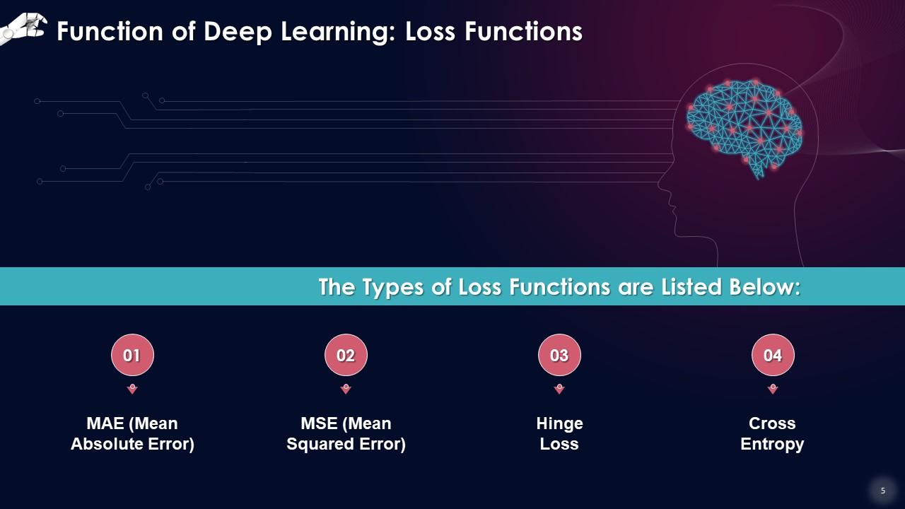
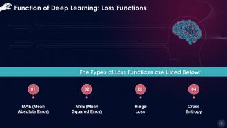
This slide lists the types of loss functions as a component of Deep Learning. These include mean absolute error, mean squared error, hinge loss, and cross-entropy.
Slide 6
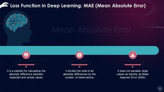
This slide states that mean absolute error is a statistic for calculating the absolute difference between expected and actual values. Divide the total of all absolute differences by the number of observations. It does not penalize large values as harshly as Mean Squared Error (MSE).
Slide 7
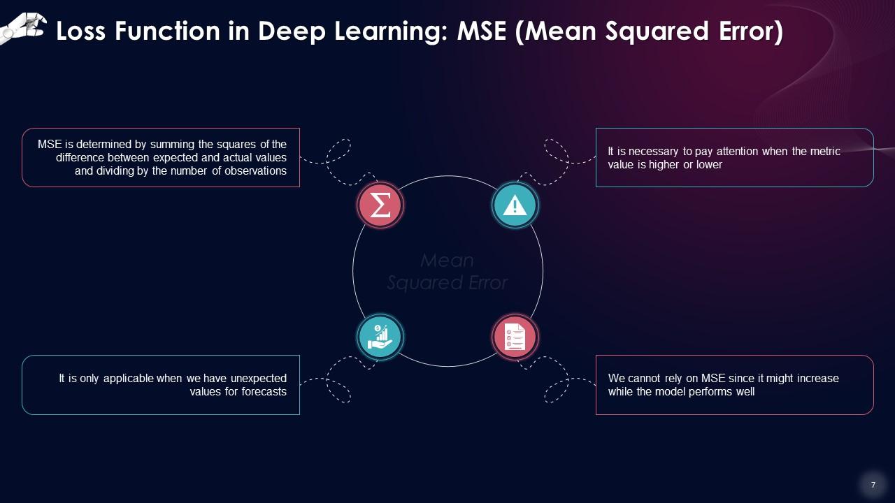
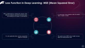
This slide describes that MSE is determined by summing the squares of the difference between expected and actual values and dividing by the number of observations. It is necessary to pay attention when the metric value is higher or lower. It is only applicable when we have unexpected values for forecasts. We cannot rely on MSE since it might increase while the model performs well.
Slide 8
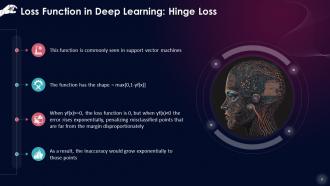
This slide explains that hinge loss function is commonly seen in support vector machines. The function has the shape = max[0,1-yf(x)]. When yf(x)>=0, the loss function is 0, but when yf(x)<0 the error rises exponentially, penalizing misclassified points that are far from the margin disproportionately. As a result, the inaccuracy would grow exponentially to those points.
Slide 9
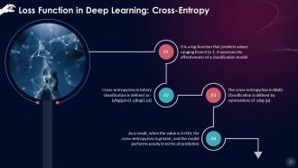
This slide states that cross-entropy is a log function that predicts values ranging from 0 to 1. It assesses the effectiveness of a classification model. As a result, when the value is 0.010, the cross-entropy loss is more significant, and the model performs poorly on prediction.
Slide 10
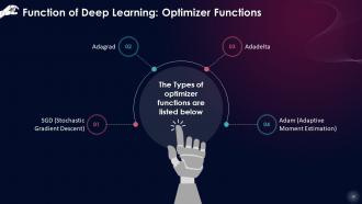
This slide lists optimizer functions as a part of Deep Learning. These include stochastic gradient descent, adagrad, adadelta and adam (adaptive moment estimation).
Slide 11
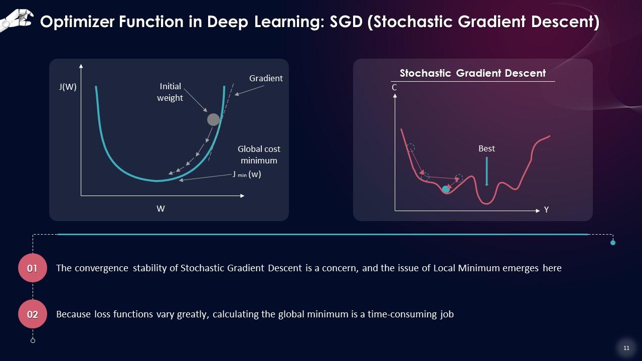
This slide states that the convergence stability of Stochastic Gradient Descent is a concern, and the issue of Local Minimum emerges here. With loss functions varying greatly, calculating the global minimum is time-consuming.
Slide 12
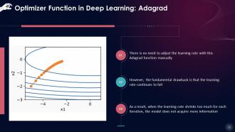
This slide states that there is no need to adjust the learning rate with this Adagrad function manually. However, the fundamental drawback is that the learning rate continues to fall. As a result, when the learning rate shrinks too much for each iteration, the model does not acquire more information.
Slide 13
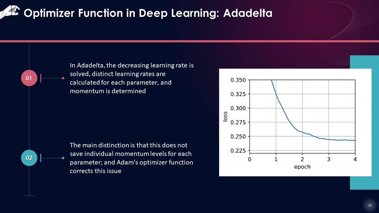
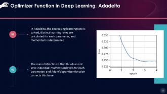
This slide states that in adadelta, the decreasing learning rate is solved, distinct learning rates are calculated for each parameter, and momentum is determined. The main distinction is that this does not save individual momentum levels for each parameter; and Adam's optimizer function corrects this issue.
Slide 14
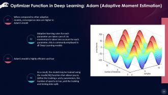
This slide describes that when compared to other adaptive models, convergence rates are higher in Adam's model. Adaptive learning rates for each parameter are taken care of. As momentum is taken into account for each parameter, this is commonly employed in all Deep Learning models. Adam's model is highly efficient and fast.
Core Functions Of Deep Learning Training Ppt with all 30 slides:
Use our Core Functions Of Deep Learning Training Ppt to effectively help you save your valuable time. They are readymade to fit into any presentation structure.
-
Their designing team is so expert in making tailored templates. They craft the exact thing I have in my mind…..really happy.
-
The website is jam-packed with fantastic and creative templates for a variety of business concepts. They are easy to use and customize.


