

Essentials Of Artificial Neural Networks Training Ppt





Try Before you Buy Download Free Sample Product
 Impress Your
Audience
 100%
Editable
 Save Hours
of Time


These slides discuss the concept of artificial neural networks. There are three layers in the neural network the input layer, the hidden layer, and the output layer. The activation function is used to calculate a weighted total and then add bias to it to determine whether a neuron should be activated or not. It also describes the working of a neural network. It also explains gradient descent and backpropagation.
People who downloaded this PowerPoint presentation also viewed the following :
Content of this Powerpoint Presentation
Slide 1
This slide depicts a separator slide for the session introduction to sales fundamentals.
Slide 2
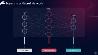
This slide depicts the layers in a Neural network. There are three layers known as the input layer, hidden layer, and output layer.
Instructor’s Notes:
- Input Layer: The input layer comes first. This layer will accept the data, which will then send it to the remainder of the network
- Hidden Layer: The hidden layer is the second of the three layers. A neural network’s hidden layers can be one or more in number. The hidden layers are the ones that are accountable for neural networks' high performance and complexity. They may do a number of tasks at once, such as data transformation, automatic feature development, etc
- Output Layer: The output layer is the final layer. The outcome or output of the problem is stored in the output layer. The input layer receives raw photos, and the output layer delivers the final version of the result
Slide 3
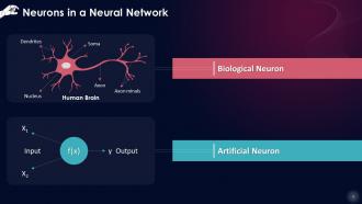
This slide illustrates the artificial neurons present in the layers of an Artificial Neural Network (ANN). It draws a comparison between the biological neurons present in human brains with an artificial neuron in an ANN.
Instructor’s Notes: A layer is made up of microscopic units known as neurons. A neuron in a neural network can be better understood with the help of biological neurons. An artificial neuron is analogous to a biological neuron. It takes information from other neurons, processes it, and then produces an output. Here, X1 and X2 are the artificial neurons' inputs, f(X) is the processing done on the inputs, and y is the neuron's output.
Slide 4
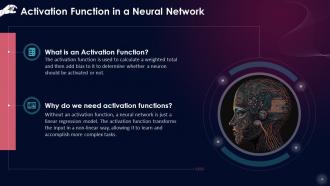
This slide gives an introduction to activation function in a neural network and discusses its importance. The activation function is used to calculate a weighted total and then add bias to it to determine whether a neuron should be activated or not.
Slide 5
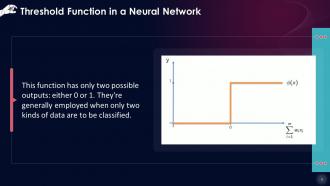
This slide illustrates Threshold Function which is a type of Activation Function in a neural network. This function has only two possible outputs: either 0 or 1. They're generally employed when only two kinds of data are to be classified.
Slide 6
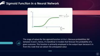
This slide depicts Sigmoid Function which is a type of activation function. The range of values for the sigmoid function is 0 to 1. This function is primarily employed in the output layer because it is from this node that we obtain the anticipated value
Slide 7
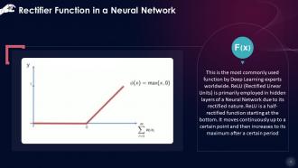
This slide illustrates Rectifier or ReLU function which is a type of activation function. Relu (Rectified Linear Units) is primarily employed in hidden layers of a Neural Network due to its rectified nature. Relu is a half-rectified function starting at the bottom. It moves continuously up to a certain point and then increases to its maximum after a certain period
Slide 8
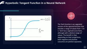
This slide depicts Hyperbolic Tangent Function which is a type of activation function. The Tanh function is an upgraded version of the sigmoid function that includes a range of values from -1 to 1. Tanh has a sigmoid curve form, although with a distinct range of values. The benefit is that, depending on their projections, both negative and positive outcomes are plotted separately
Slide 9
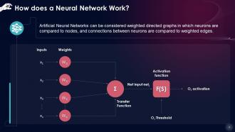
This slide describes the working of an Artificial Neural Network. Artificial Neural Networks can be considered weighted directed graphs in which neurons are compared to nodes, and connections between neurons are compared to weighted edges.
Instructor’s Notes: A neuron's processing element receives many signals, which are occasionally altered at the receiving synapse before being summed at the processing element. If it reaches the threshold, it becomes an input to other neurons, and the cycle begins again
Slide 10
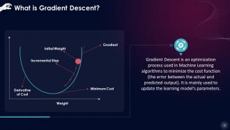
This slide introduces the concept of gradient descent. Gradient Descent is an optimization process used in Machine Learning algorithms to minimize the cost function (the error between the actual and predicted output). It is mainly used to update the learning model's parameters.
Slide 11
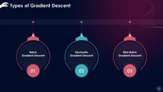
This slide lists types of gradient descent. These include batch gradient descent, stochastic gradient descent, and mini-batch gradient descent.
Instructor’s Notes:
- Batch Gradient Descent: Batch gradient descent adds the errors for each point in a training set before updating the model after all training instances have been reviewed. This process is known as the Training Epoch. Batch gradient descent usually gives a steady error gradient and convergence, although choosing the local minimum rather than the global minimum isn't always the best solution
- Stochastic Gradient Descent: Stochastic gradient descent creates a training epoch for each example in the dataset and changes the parameters of each training example, sequentially. These frequent updates can provide greater detail and speed, but they can also produce noisy gradients, which can aid in surpassing the local minimum and locating the global one
- Mini-Batch Gradient Descent: Mini-batch gradient descent combines the principles of both batch gradient descent with stochastic gradient descent. It divides the training dataset into distinct groups and updates them separately. This method balances batch gradient descent's computing efficiency and stochastic gradient descent's speed
Slide 12
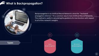
This slide describes the concept of backpropagation along with its two types that are Static backpropagation and Recurrent backpropagation. Backpropagation is useful in calculating the gradient of a loss function with respect to all of the network's weights.
Instructor’s Notes:
- Static Backpropagation: The mapping of static input generates a static output in this type of backpropagation. It is used to address challenges like optical character recognition that requires static classification
- Recurrent Backpropagation: The Recurrent Propagation is directed forward or conducted till a specific set value, or threshold value is attained. The error is evaluated and propagated backward after reaching a particular value
Slide 13
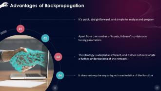
This slide lists the advantages of Backpropagation. These are that it is simple & straightforward, adaptable & efficient, and it does not require any unique characteristics.
Slide 14
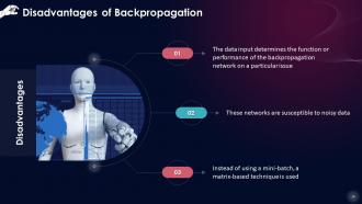
This slide lists the disadvantages of Backpropagation. These are that the data input determines the function of the entire network on a particular issue, networks are susceptible to noisy data, and a matrix based technique is used.
Slide 15
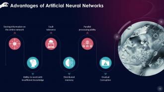
This slide lists the advantages of Artificial Neural Networks. These advantages include that ANN stores information on the entire network, its ability to work with insufficient knowledge, its fault tolerance, a distributed memory, and parallel processing ability.
Instructor’s Notes:
- Storing information on the entire network: Information is saved on the entire network, not in a database, as done in traditional programming. The network continues to function despite losing a few pieces of information in one location
- Ability to work with insufficient knowledge: After training the Artificial Neural Network, the data can yield output even with limited or insufficient information
- Fault tolerance: The output of an ANN is unaffected by the corruption of one or more of its cells. The networks become fault-tolerant as a result of this characteristic
- Distributed memory: It is required to determine the examples and train the network according to the intended output. The network's progress is proportional to the instances chosen. If the event cannot be displayed to the network in all aspects, it may generate inaccurate results
- Parallel processing ability: Artificial Neural Networks have the computational power to perform multiple tasks at once
- Gradual Corruption: The network is not immediately corroded as its performance degrades and slows over time.
Slide 16
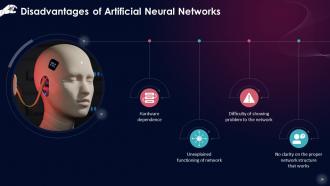
This slide lists the disadvantages of Artificial Neural Networks. These disadvantages include ANNs’ hardware dependence, unexplained functioning of network, difficulty of showing problem to the network, and no clarity on the proper network structure that works.
Instructor’s Notes:
- Hardware dependence: The structure of Artificial Neural Networks necessitates parallel processing power. As a result, the implementation is equipment dependent
- Unexplained functioning of network: When ANN provides a probing solution, it does not explain why or how it was chosen. This decreases trust in the network
- Difficulty of showing problem to the network: ANNs are able to work with numerical data. Before introducing ANN to a problem, it must be transformed into numerical values. The display mechanism chosen here will directly impact the network's performance, depending on the user's skill level
- No clarity on the proper network structure that works: No explicit rule determines the structure of artificial neural networks. Experience and trial & error are used to create the ideal network structure
Essentials Of Artificial Neural Networks Training Ppt with all 32 slides:
Use our Essentials Of Artificial Neural Networks Training Ppt to effectively help you save your valuable time. They are readymade to fit into any presentation structure.

















FAQs for Essentials Of Artificial Neural
So basically you've got neurons (the nodes) connected in layers - input layer takes your data, hidden layers do all the heavy lifting, then output spits out results. Each connection has weights that control how strong the signal is, and that's where all the learning magic happens during training. Think of neurons like tiny decision-makers that either "fire" or stay quiet based on their activation function. The tricky part is figuring out how many hidden layers you actually need - honestly depends on how complex your problem is. Oh and the weights between connections? That's literally what makes or breaks your whole network.
So basically backpropagation figures out which weights screwed up your prediction and by how much. It starts at the output layer and works backwards through each layer - kinda like detective work but with calculus. The chain rule helps you calculate gradients for every weight, then gradient descent updates them to reduce error. Honestly took me forever to get this concept when I first learned it. Short version: you're tracing responsibility backwards through the network. I'd definitely start with just two layers first - the math gets wild once you add more depth, trust me.
So learning rate is basically how big steps your model takes when updating weights - like the "speed" it learns at. Go too high? Your model bounces around like crazy and never settles on the right answer. Too low and it'll take forever, might even get stuck. Honestly such a pain to get right lol. You want steady loss decrease without wild swings. I usually start with 0.001 or 0.01, then mess around with schedules that slow down over time. Works way better for fine-tuning that way.
Oh yeah, overfitting is annoying but totally fixable. Dropout is your best friend - try 0.2 to 0.5 and it randomly shuts off neurons so your model can't just memorize everything. Early stopping works great too, just watch when validation loss starts climbing while training loss keeps dropping. That's when you know to quit. More data always helps if you can swing it, or try data augmentation to fake having more. Cross-validation gives you a better picture of what's actually happening. Honestly, I'd start with dropout and early stopping since they're pretty foolproof.
Imbalanced data is such a pain, but there's a few things that actually work. Class weighting is probably your best starting point - it just makes the model care more about getting the minority class right. SMOTE is solid for creating synthetic examples of your rare class, or you could undersample the majority one instead. Focal loss is pretty neat too since it makes the model focus on the tricky examples it keeps getting wrong. Oh, and ensemble methods can be surprisingly good at this stuff. I'd honestly just start with adjusting class weights first since it's super easy to code up, then see how your precision/recall looks.
Honestly, just go with ReLU - it's the safe choice that actually works. I wasted so much time overthinking this on my first project lol. The thing is, sigmoid and tanh sound fancy but they'll kill your gradients in deeper networks. ReLU keeps things flowing so your early layers don't get stuck with tiny updates. Dead neurons bugging you? Try Leaky ReLU or ELU, but that's usually overkill. Don't get cute with exotic functions unless ReLU is clearly failing you. Trust me, vanilla ReLU handles like 90% of cases perfectly fine.
So batch size is just how many samples your model looks at before updating its weights. Small batches = noisy updates but they happen more often. Big batches are smoother but eat up way more memory (plus they can get trapped in weird spots sometimes). Most people stick with powers of 2 - like 32, 64, 128. Honestly, I'd just start with 32 and mess around from there. Watch your training speed and see if it's actually learning properly. Your hardware will probably dictate a lot of this anyway.
Honestly, transfer learning is a game changer - you basically grab a pre-trained model that's already learned stuff on huge datasets, then just fine-tune it for your specific problem. Way faster than starting from zero. The model already knows basic patterns like edges and shapes, so you're not teaching it everything from scratch. Perfect when your data is limited (which... yeah, happens a lot). You can either freeze those early layers and just retrain the last few, or fine-tune everything with a really low learning rate. Saves so much time and usually works better too.
Honestly, the biggest pain points are vanishing/exploding gradients and overfitting. Deep networks either kill your gradients completely or they blow up - both mess with training. Your model will also memorize the training data instead of actually learning patterns, which is annoying. Local minima are another headache where you get stuck in okay solutions instead of great ones. Hyperparameter tuning is basically just suffering through endless experiments until something works. Weight initialization helps a ton, and dropout or batch normalization can save you. Always test on fresh data though - that's how you'll catch problems early.
Oh definitely normalize your data! Your network will thank you for it. Without normalization, features with bigger numbers basically bully the smaller ones during training. Like if you're comparing salaries vs age - the salary numbers are way bigger so the model thinks they're more important. I usually go with z-score normalization but min-max works too. The tricky part is making sure you use the same scaling on your test data as your training data. Otherwise you're kinda cheating. Your gradients flow way better with normalized data and training actually converges instead of getting stuck in weird spots.
Depends what you're building, honestly. Classification? Go with accuracy, precision, recall, F1-score. Regression needs MSE, RMSE, MAE. I'm weird about checking loss curves constantly - they'll show if you're overfitting way before anything else does. Training metrics lie though. Your validation and test performance is what actually matters. Oh, and if your data's imbalanced, accuracy becomes totally useless. Stick with precision/recall or AUC-ROC instead. Plot everything over epochs and use multiple metrics together - gives you the real story of what's happening.
So basically regularization stops your model from just memorizing training data instead of actually learning patterns. It's like studying for a test - you want to understand the concepts, not memorize every single practice question, you know? Dropout and L2 regularization add constraints that force the model to learn more general stuff. Try dropout first (like 0.2-0.5 rate) - it's super easy to implement and usually helps right away. L2 is solid too. Both punish overly complex models that get too obsessed with fitting training examples perfectly, which honestly makes them way better on new data.
So basically, supervised learning is when you show the algorithm examples with the "right answers" - like photos labeled "cat" or "dog." It learns from those. Unsupervised is way messier because you just dump raw data on it and hope it finds patterns. No labels, no guidance. It might group similar customers together or spot weird outliers. Supervised works great when you know what you're looking for. Unsupervised is better for discovering stuff you didn't even know was there - though honestly it can be a pain to interpret sometimes.
So hyperparameter tuning is basically finding that sweet spot where your model learns at just the right pace - not too fast, not too slow. Honestly, it's one of those things that seems tedious but saves you tons of time later. Your learning rate and batch size? Start there, they'll give you the most noticeable improvements. Without decent tuning, you'll just sit there watching your loss function do weird bouncy things for hours (been there). Think of it like adjusting a recipe - small tweaks make everything work way better. The whole thing really does cut down training time once you get it dialed in.
Honestly, adaptive optimizers changed everything. Adam's probably your best bet to start with - it handles momentum and adjusts learning rates automatically, so you're not constantly tweaking that one annoying hyperparameter. Before Adam and stuff like RMSprop came around, people would waste so much time on manual tuning. Training's way more stable now and converges faster too. There's also AdamW if you run into weight decay problems later. I'd say just go with Adam first since it works well right out of the box, then maybe experiment if you need better performance. Works for like 90% of cases anyway.
-
I was able to find the right choice of PPT template for my thesis with SlideTeam. Thank you for existing.
-
The website is jam-packed with fantastic and creative templates for a variety of business concepts. They are easy to use and customize.